The UTSA School of Music cultivates innovation, artistry, and scholarship while amplifying the cultural wealth of San Antonio and enriching our community through music and performing arts. We empower students by nurturing their musicianship, integrating their personal values and goals into their professional identities, and fostering discovery and growth.
The University of Texas at San Antonio is accredited by the National Association of Schools of Music.

Contact
Interim Director of UTSA Arts , Special Assistant to the Dean for Community Engagement and the Arts, Roland K. Blumberg Endowed Professor in Music
tracy.cowden@utsa.edu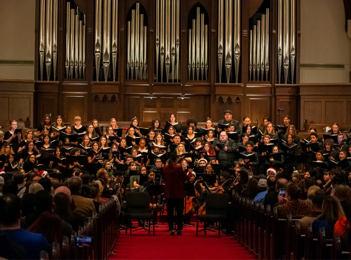
The Verdi Project
Friday, April 26 at 7:00 PM
Edgewood Theatre of Performing Arts
Don't miss this one-night-only spectacle! As a part of its 50th Anniversary celebration, the UTSA School of Music presents a collaboration between the UTSA Choirs, Lyric Theatre, and Orchestra. Join us for an evening featuring the operatic music of Giuseppe Verdi. The performance tells the life story of the Italian composer through the lens of his own music.
School of Music Events
View All EventsHave an inquiry about UTSA School of Music?
We appreciate your interest and extend our warmest welcome to you from the School of Music.
Apply to Audition
All prospective transfer students are required to take a theory exam on their audition day. Incoming freshmen do not take theory exams.
School of Music Degree Programs
See all the degrees available from the UTSA School of Music
Book Us
To request a UTSA School of Music Performance, please follow this link to submit a request form.
UTSA School of Music Digital Magazines


Latest News
Read All News Stories

January 17, 2024
Linda Jenkins To Perform UTSA Faculty Debut In The Hall on FridayThe performance is set to be the second iteration of the UTSA School of Music's Maestría Faculty Artist Series, an initiative and branding launched in October 2023 to promote public interest in UTSA faculty artist performances. Jenkins' performance is the first of five new entries in the concert series that will be announced soon. Jenkins is joined by the school's collaborative pianist, Dr. Jeong Eun-Lee, who has been with the school since August 2022.
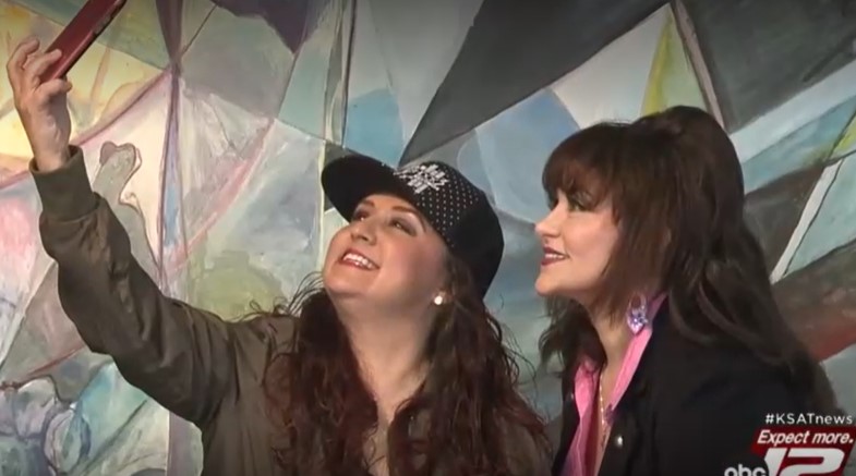
January 3, 2024
Tejano music pioneers expand their horizons in surprising waysShelly Lares and Patsy Torres each decided to build on their celebrity in ways some of their devoted fans may find surprising after making their marks in the Tejano music industry that they helped pioneer.